The Fourier transform, explained the way it finally clicked

Almost everyone meets the Fourier transform as a wall of integrals. That's backwards — the idea is simple and the notation is the hard part. We'll do the idea first, then earn the details.

One honest sentence

Here is the whole thing in plain words: any signal can be rebuilt by adding together plain sine waves of different frequencies, amplitudes and offsets. The Fourier transform is nothing more than the recipe that tells you which sine waves you need, and how much of each. That's it. Everything else — the integrals, the complex exponentials, the notation that makes textbooks look intimidating — is machinery built around that one idea.

If you can accept that a musical chord is several pure notes played at once, you already have the intuition. A microphone records the chord as a single wiggling line: the sum of all those notes added together, moment by moment. Your ear does the reverse — it pulls that one line apart and lets you hear the individual notes inside it. The Fourier transform does exactly the same pulling-apart, with mathematics instead of a cochlea. It takes the wiggle and hands you back the list of pure tones that, added together, reproduce it.

Two views of one object

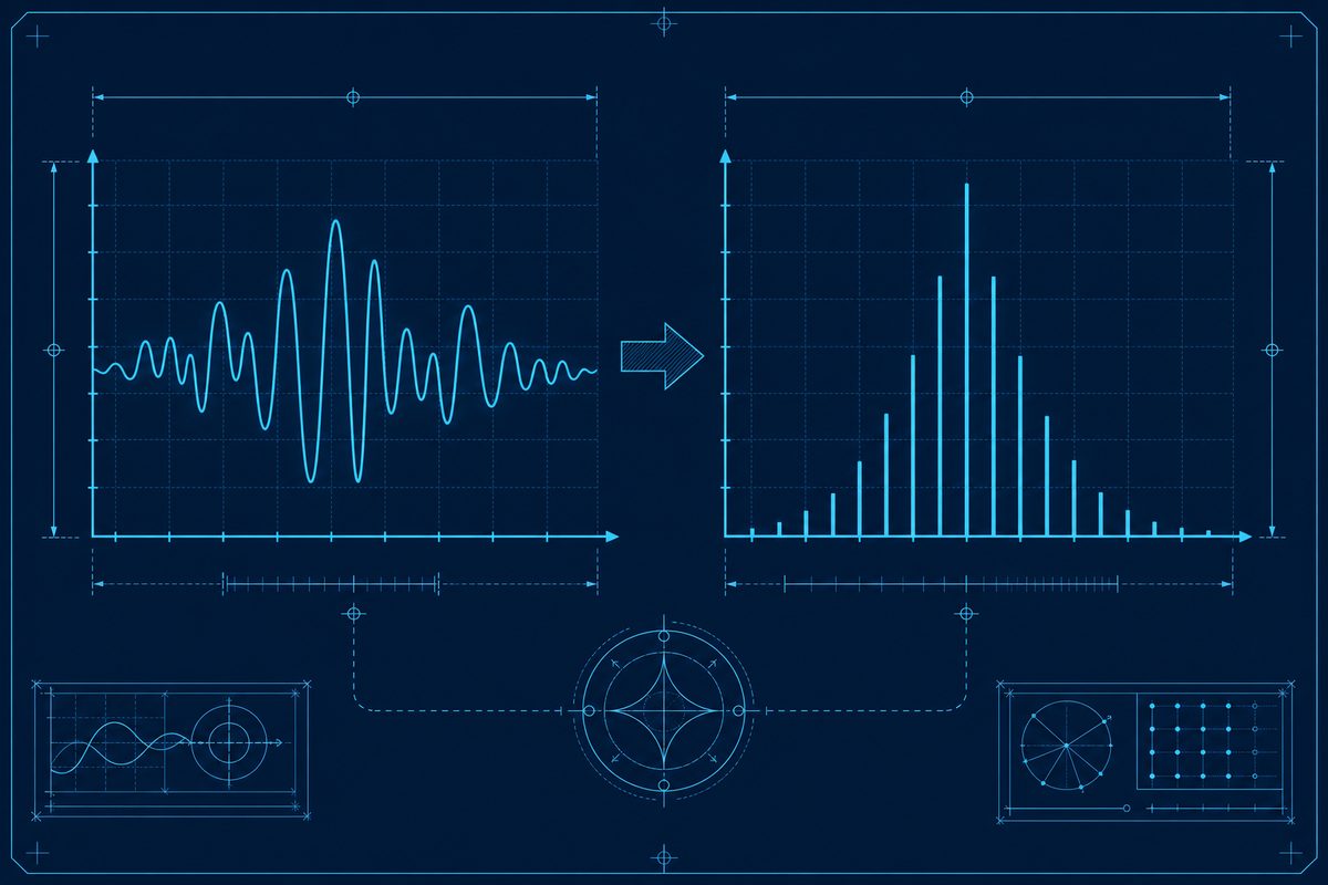
There are two ways to describe the same signal, and neither is more true than the other. In the time domain, a signal is amplitude versus time — the wiggling line you'd see on an oscilloscope. In the frequency domain, the same signal is amplitude versus frequency — a set of bars that say “this much energy at 440 Hz, this much at 880 Hz, nothing at 1000 Hz.”

The frequency domain is not a different signal. It is the same signal, seen from the side.

Think of a glass prism. White light goes in; a rainbow comes out. The prism didn't add anything — the colours were always present in the white light, just summed together into something that looked colourless. The prism unstacks them. The Fourier transform is a prism for signals: it takes something that looks like a featureless wiggle and shows you the spectrum of frequencies that were hiding inside it the whole time.

Why anyone bothers leaving the time domain

Here is the payoff that makes the whole apparatus worth learning: operations that are painful in the time domain become almost trivial in the frequency domain. Suppose your audio recording has an annoying 60 Hz hum from mains electricity buzzing underneath everything. In the time domain, removing it means designing and applying a filter — a fiddly convolution that's easy to get wrong. In the frequency domain, you transform the signal, look at the bar sitting at 60 Hz, set it to zero, and transform back. The hum is gone.

This pattern repeats across engineering. Compression, noise reduction, equalisation, radio tuning, image processing, the analysis of vibrations in a bridge or an engine — an enormous fraction of practical work is just choosing the domain in which the problem is easy and doing the work there. The Fourier transform is the door between the two rooms.

A minimal worked example

Make a signal that is one part of a 2 Hz sine wave plus half a part of a 5 Hz sine wave. Plot it in time and you get a lumpy, irregular-looking wave that you'd struggle to describe in words. Now run a discrete Fourier transform over a few seconds of it. The output is almost boringly clean: a tall spike at exactly 2 Hz, and a spike half as tall at exactly 5 Hz, and essentially nothing anywhere else. The transform read the recipe straight off the wiggle — two ingredients, in the exact proportions we used.

In code, the discrete version is a single function call — in Python, numpy.fft.rfft(signal). But the call is not the lesson. The lesson is what the output means: each element (each “bin”) corresponds to a specific frequency, and its magnitude tells you how much of that frequency is present. The list of bins is your spectrum.

The two knobs that trip everyone up

Two practical facts cause the majority of real-world confusion, and both come from the fact that we work with sampled, finite signals rather than perfect continuous ones.

First, sampling rate sets the ceiling on what you can see. If you sample a signal 1000 times per second, the highest frequency you can faithfully represent is 500 Hz — half the sample rate, a limit called the Nyquist frequency. Push a higher frequency into a system sampling too slowly and it doesn't just disappear; it folds back down and masquerades as a lower frequency that isn't really there. This is aliasing, and it's the reason wagon wheels appear to spin backwards in old films and why anti-aliasing filters exist in every audio interface. If your spectrum shows energy where you know there shouldn't be any, aliasing is the first suspect.

Second, how long you record sets your resolution. Frequency resolution — your ability to tell 100 Hz apart from 101 Hz — depends on the length of the recording, not the sample rate. A very short clip simply hasn't watched the signal long enough to distinguish two nearby frequencies; they smear into one blurry bump. Want to resolve fine frequency detail? Record for longer. There's no free lunch: sharp frequency resolution costs you time resolution, and vice versa.

Where the clean story breaks

The tidy picture — signal in, spectrum out — quietly assumes that the frequency content of your signal doesn't change over the window you analyse. For a pure tone or a stationary hum, fine. But real signals almost never hold still. Speech is a rapid sequence of different sounds. Music changes chord. A machine's vibration signature shifts as it heats up or wears down. Run one giant Fourier transform over a three-minute song and you get the average spectrum of the entire song — technically correct and almost useless, because it's tells you nothing about when each frequency happened.

The fix is the spectrogram. Instead of one transform over the whole signal, you chop the signal into short, overlapping windows and transform each one separately. Now you have frequency content over time — a two-dimensional picture where the horizontal axis is time, the vertical axis is frequency, and brightness shows energy. This is what you see in audio editors and voice-analysis tools, and it's the honest instrument for any signal that won't sit still. It's also the natural next step the moment the plain transform clicks, which is exactly why we introduce the plain transform first.

What to carry away

Don't try to memorise the integral — it's the compressed form, and memorising a compression without understanding what it compresses is how people end up afraid of this topic for years. Carry the sentence instead: a signal is a sum of waves, and the transform hands you the list of waves. Bins, Nyquist, aliasing, resolution, windowing, the spectrogram — every one of them is bookkeeping around that single idea. Get the idea solid and the machinery stops being intimidating and starts being obvious.

Found an error? Tell us — corrections improve the register.